
티스토리 뷰
2024.03.25
클라우드 기반의 디지털 콘텐츠 스트리밍과 인코딩 수업
plt.imshow(image, cmap="gray"), plt.axis("off")
plt.show()
!mkdir imagesimport cv2
import numpy as np
from matplotlib import pyplot as plt
image = cv2.imread("images/plane.jpg", cv2.IMREAD_GRAYSCALE)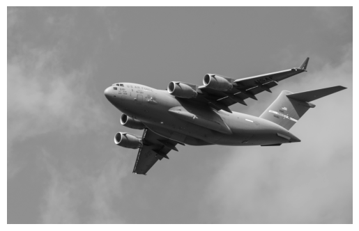
type(image)
#numpy.ndarrayimage
'''
image
array([[140, 136, 146, ..., 132, 139, 134],
[144, 136, 149, ..., 142, 124, 126],
[152, 139, 144, ..., 121, 127, 134],
...,
[156, 146, 144, ..., 157, 154, 151],
[146, 150, 147, ..., 156, 158, 157],
[143, 138, 147, ..., 156, 157, 157]], dtype=uint8)
'''image.shape
#(2270, 3600)image[0]
#array([140, 136, 146, ..., 132, 139, 134], dtype=uint8)image[0][3599]
#134image_bgr = cv2.imread("images/plane.jpg", cv2.IMREAD_COLOR)
image_bgr[0,0]
#array([195, 144, 111], dtype=uint8)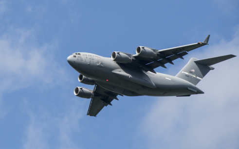
import cv2
import numpy as np
from matplotlib import pyplot as plt

image = cv2.imread("images/plane.jpg", cv2.IMREAD_GRAYSCALE)
cv2.imwrite("images/plane_new.jpg", image)
#True!wget https://github.com/rickiepark/machine-learning-with-python-cookbook/raw/master/images/plane_256x256.jpg -O images/plane_256x256.jpgimport cv2
import numpy as np
from matplotlib import pyplot as plt
# 흑백 이미지로 로드합니다.
image = cv2.imread("images/plane_256x256.jpg", cv2.IMREAD_GRAYSCALE)image_50x50 = cv2.resize(image, (50, 50))
plt.imshow(image_50x50, cmap="gray"), plt.axis("off")
plt.show
import cv2
import numpy as np
from matplotlib import pyplot as plt

# 흑백 이미지로 로드합니다.
image = cv2.imread("images/plane_256x256.jpg", cv2.IMREAD_GRAYSCALE)
image_cropped = image[:,:128]
plt.imshow(image_cropped, cmap="gray"), plt.axis("off")
plt.show()
import cv2
import numpy as np
from matplotlib import pyplot as plt

# 흑백 이미지로 로드합니다.
image = cv2.imread("images/plane_256x256.jpg", cv2.IMREAD_GRAYSCALE)

image_blurry = cv2.blur(image, (10,10))

plt.imshow(image_blurry, cmap="gray"), plt.axis("off")
plt.show()
image_very_blurry = cv2.blur(image, (100,100))

plt.imshow(image_very_blurry, cmap="gray"), plt.xticks([]), plt.yticks([])
plt.show()
kernel = np.ones((5,5)) / 25.0kernel
'''
array([[0.04, 0.04, 0.04, 0.04, 0.04],
[0.04, 0.04, 0.04, 0.04, 0.04],
[0.04, 0.04, 0.04, 0.04, 0.04],
[0.04, 0.04, 0.04, 0.04, 0.04],
[0.04, 0.04, 0.04, 0.04, 0.04]])
'''image_kernel = cv2.filter2D(image, -1, kernel)
plt.imshow(image_kernel, cmap="gray"), plt.xticks([]), plt.yticks([])
plt.show()
image_very_blurry = cv2.GaussianBlur(image, (5,5), 0)

plt.imshow(image_very_blurry, cmap="gray"), plt.xticks([]), plt.yticks([])
plt.show()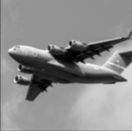
gaus_vector = cv2.getGaussianKernel(5,0)
gaus_vector
'''
array([[0.0625],
       [0.25  ],
       [0.375 ],
       [0.25  ],
       [0.0625]])
'''
gaus_kernel = np.outer(gaus_vector, gaus_vector) #외접??
gaus_kernel
'''
array([[0.00390625, 0.015625 , 0.0234375 , 0.015625 , 0.00390625],
[0.015625 , 0.0625 , 0.09375 , 0.0625 , 0.015625 ],
[0.0234375 , 0.09375 , 0.140625 , 0.09375 , 0.0234375 ],
[0.015625 , 0.0625 , 0.09375 , 0.0625 , 0.015625 ],
[0.00390625, 0.015625 , 0.0234375 , 0.015625 , 0.00390625]])
'''image_kernel = cv2.filter2D(image, -1, gaus_kernel)
plt.imshow(image_kernel, cmap="gray"), plt.xticks([]), plt.yticks([])
plt.show()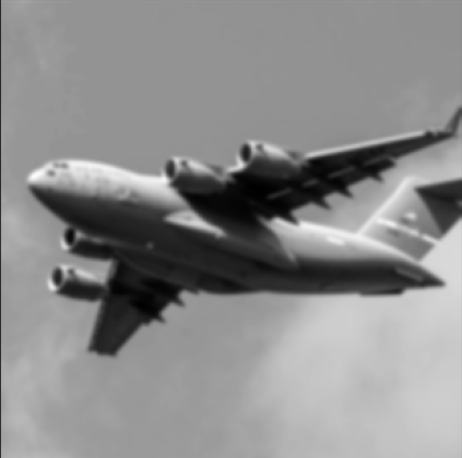
import cv2
import numpy as np
from matplotlib import pyplot as plt

# 흑백 이미지로 로드합니다.
image = cv2.imread("images/plane_256x256.jpg", cv2.IMREAD_GRAYSCALE)

kernel = np.array([[0,-1,0],
                  [-1,5,-1],
                  [0,-1,0]])

image_sharp = cv2.filter2D(image, -1, kernel)

plt.imshow(image_sharp, cmap="gray"), plt.axis("off")
plt.show()
import cv2
import numpy as np
from matplotlib import pyplot as plt

# 흑백 이미지로 로드합니다.
image = cv2.imread("images/plane_256x256.jpg", cv2.IMREAD_GRAYSCALE)

image_enhanced = cv2.equalizeHist(image)

plt.imshow(image_enhanced, cmap="gray"), plt.axis("off")
plt.show()
import cv2
import numpy as np
from matplotlib import pyplot as plt

image_bgr = cv2.imread("images/plane_256x256.jpg")

image_yuv = cv2.cvtColor(image_bgr, cv2.COLOR_BGR2YUV)

image_yuv[:,:,0] = cv2.equalizeHist(image_yuv[:,:,0])

image_rgb = cv2.cvtColor(image_yuv, cv2.COLOR_YUV2RGB)

plt.imshow(image_rgb, cmap="gray"), plt.axis("off")
plt.show()
import cv2
import numpy as np
from matplotlib import pyplot as plt

image_bgr = cv2.imread("images/plane_256x256.jpg")

image_hsv = cv2.cvtColor(image_bgr, cv2.COLOR_BGR2HSV)

lower_blue = np.array([50,100,50])
upper_blue = np.array([130,255,255])

mask = cv2.inRange(image_hsv, lower_blue, upper_blue)

image_bgr_masked = cv2.bitwise_and(image_bgr, image_bgr, mask=mask)

image_rgb = cv2.cvtColor(image_bgr_masked, cv2.COLOR_BGR2RGB)

plt.imshow(image_rgb), plt.axis("off")
plt.show()
plt.imshow(mask, cmap="gray"), plt.axis("off")
plt.show()
import cv2
import numpy as np
from matplotlib import pyplot as plt

image_grey = cv2.imread("images/plane_256x256.jpg", cv2.IMREAD_GRAYSCALE)

max_output_value = 255
neighborhood_size = 99
subtract_from_mean = 10

image_binarized = cv2.adaptiveThreshold(
    image_grey,
    max_output_value,
    cv2.ADAPTIVE_THRESH_GAUSSIAN_C,
    cv2.THRESH_BINARY,
    neighborhood_size,
    subtract_from_mean
)

plt.imshow(image_binarized), plt.axis("off")
plt.show()
image_binarized = cv2.adaptiveThreshold(
    image_grey,
    max_output_value,
    cv2.ADAPTIVE_THRESH_MEAN_C,
    cv2.THRESH_BINARY,
    neighborhood_size,
    subtract_from_mean
)

plt.imshow(image_binarized), plt.axis("off")
plt.show()
import cv2
import numpy as np
from matplotlib import pyplot as plt

image_bgr = cv2.imread("images/plane_256x256.jpg")
image_rgb = cv2.cvtColor(image_bgr, cv2.COLOR_BGR2RGB)

rectangle = (0, 56, 256, 150)

mask = np.zeros(image_rgb.shape[:2], np.uint8)

bgdModel = np.zeros((1,65), np.float64)
fgdModel = np.zeros((1,65), np.float64)

cv2.grabCut(
    image_rgb,
    mask,
    rectangle,
    bgdModel,
    fgdModel,
    5,
    cv2.GC_INIT_WITH_RECT
)

mask_2 = np.where((mask==2) | (mask==0), 0, 1).astype('uint8')

image_rgb_nobg = image_rgb * mask_2[:, :, np.newaxis]


plt.imshow(image_rgb_nobg), plt.axis("off")
plt.show()
# 라이브러리를 임포트합니다.
import cv2
import numpy as np
from matplotlib import pyplot as plt

# 흑백 이미지로 로드합니다.
image_gray = cv2.imread("images/plane_256x256.jpg", cv2.IMREAD_GRAYSCALE)

# 픽셀 강도의 중간값을 계산합니다.
median_intensity = np.median(image_gray)

# 중간 픽셀 강도에서 위아래 1 표준 편차 떨어진 값을 임계값으로 지정합니다.
lower_threshold = int(max(0, (1.0 - 0.33) * median_intensity))
upper_threshold = int(min(255, (1.0 + 0.33) * median_intensity))

# 캐니 경계선 감지기를 적용합니다.
image_canny = cv2.Canny(image_gray, lower_threshold, upper_threshold)

# 이미지를 출력합니다.
plt.imshow(image_canny, cmap="gray"), plt.axis("off")
plt.show()
# 라이브러리를 임포트합니다.
import cv2
import numpy as np
from matplotlib import pyplot as plt

# 흑백 이미지로 로드합니다.
image_bgr = cv2.imread("images/plane_256x256.jpg")
image_gray = cv2.cvtColor(image_bgr, cv2.COLOR_BGR2GRAY)
image_gray = np.float32(image_gray)

# 모서리 감지 매개변수를 설정합니다.
block_size = 2
aperture = 29
free_parameter = 0.04

# 모서리를 감지합니다.
detector_responses = cv2.cornerHarris(image_gray,
                                      block_size,
                                      aperture,
                                      free_parameter)

# 모서리 표시를 부각시킵니다.
detector_responses = cv2.dilate(detector_responses, None)

# 임계값보다 큰 감지 결과만 남기고 흰색으로 표시합니다.
threshold = 0.02
image_bgr[detector_responses >
          threshold *
          detector_responses.max()] = [255,255,255]

# 흑백으로 변환합니다.
image_gray = cv2.cvtColor(image_bgr, cv2.COLOR_BGR2GRAY)

# 이미지를 출력합니다.
plt.imshow(image_gray, cmap="gray"), plt.axis("off")
plt.show()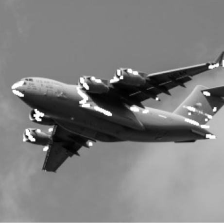
plt.imshow(detector_responses, cmap='gray'), plt.axis("off")
plt.show()
# 이미지를 로드합니다.
image_bgr = cv2.imread('images/plane_256x256.jpg')
image_gray = cv2.cvtColor(image_bgr, cv2.COLOR_BGR2GRAY)

# 감지할 모서리 개수
corners_to_detect = 10
minimum_quality_score = 0.05
minimum_distance = 25

# 모서리를 감지합니다.
corners = cv2.goodFeaturesToTrack(image_gray,
                                  corners_to_detect,
                                  minimum_quality_score,
                                  minimum_distance)
corners = np.float32(corners)

# 모서리마다 흰 원을 그립니다.
for corner in corners:
    x, y = corner[0].astype('int')
    cv2.circle(image_bgr, (x,y), 10, (255,255,255), -1)

# 흑백 이미지로 변환합니다.
image_rgb = cv2.cvtColor(image_bgr, cv2.COLOR_BGR2GRAY)

# 이미지를 출력합니다.
plt.imshow(image_rgb, cmap='gray'), plt.axis("off")
plt.show()
# 라이브러리를 임포트합니다.
import cv2
import numpy as np
from matplotlib import pyplot as plt

# 흑백 이미지로 로드합니다.
image = cv2.imread("images/plane_256x256.jpg", cv2.IMREAD_GRAYSCALE)

image_10x10 = cv2.resize(image, (10,10))

image_10x10.flatten()

'''
array([133, 130, 130, 129, 130, 129, 129, 128, 128, 127, 135, 131, 131,
       131, 130, 130, 129, 128, 128, 128, 134, 132, 131, 131, 130, 129,
       129, 128, 130, 133, 132, 158, 130, 133, 130,  46,  97,  26, 132,
       143, 141,  36,  54,  91,   9,   9,  49, 144, 179,  41, 142,  95,
        32,  36,  29,  43, 113, 141, 179, 187, 141, 124,  26,  25, 132,
       135, 151, 175, 174, 184, 143, 151,  38, 133, 134, 139, 174, 177,
       169, 174, 155, 141, 135, 137, 137, 152, 169, 168, 168, 179, 152,
       139, 136, 135, 137, 143, 159, 166, 171, 175], dtype=uint8)
'''
# 이미지를 출력합니다.
plt.imshow(image_10x10, cmap='gray'), plt.axis("off")
plt.show()
image_10x10.shape

#(10, 10)

image_10x10.flatten().shape

#(100,)
image_color = cv2.imread("images/plane_256x256.jpg", cv2.IMREAD_COLOR)
image_color_10x10 = cv2.resize(image_color, (10,10))
image_color_10x10.flatten().shape
#채널이 3개니까...
#(300,)image_256x256_grey = cv2.imread("images/plane_256x256.jpg", cv2.IMREAD_GRAYSCALE)
image_256x256_grey.flatten().shape
#(65536,)
image_256x256_color = cv2.imread("images/plane_256x256.jpg", cv2.IMREAD_COLOR)
image_256x256_color.flatten().shape
#(196608,)# 라이브러리를 임포트합니다.
import cv2
import numpy as np
from matplotlib import pyplot as plt
# 이미지를 로드합니다.
image_bgr = cv2.imread("images/plane_256x256.jpg", cv2.IMREAD_COLOR)
# RGB로 변환합니다.
image_rgb = cv2.cvtColor(image_bgr, cv2.COLOR_BGR2RGB)
# 특성 값을 담을 리스트를 만듭니다.
features = []
# 각 컬러 채널에 대해 히스토그램을 계산합니다.
colors = ("r","g","b")
# 각 채널을 반복하면서 히스토그램을 계산하고 리스트에 추가합니다.
for i, channel in enumerate(colors):
histogram = cv2.calcHist([image_rgb], # 이미지
[i], # 채널 인덱스
None, # 마스크 없음
[256], # 히스토그램 크기
[0,256]) # 범위
features.extend(histogram)
# 샘플의 특성 값으로 벡터를 만듭니다.
observation = np.array(features).flatten()
# 처음 다섯 개의 특성을 출력합니다.
observation[0:5]
'''
array([1027., 217., 182., 146., 146.], dtype=float32)
'''image_rgb[0,0]
'''
array([107, 163, 212], dtype=uint8)
'''import pandas as pd
data = pd.Series([1, 1, 2, 2, 3, 3, 4, 5])
data.hist(grid=False)
plt.show()
# 각 컬러 채널에 대한 히스토그램을 계산합니다.
colors = ("r","g","b")

# 컬러 채널을 반복하면서 히스토그램을 계산하고 그래프를 그립니다.
for i, channel in enumerate(colors):
    histogram = cv2.calcHist([image_rgb], # 이미지
                        [i], # 채널 인덱스
                        None, # 마스크 없음
                        [256], # 히스토그램 크기
                        [0,256]) # 범위
    plt.plot(histogram, color = channel)
    plt.xlim([0,256])

# 그래프를 출력합니다.
plt.show()